How to use wildcard characters

 Wildcard characters are commonly used in some basic Excel formulas, i.e., COUNTIF, COUNTIFS, VLOOKUP, FIND AND REPLACE, SEARCH, CONDITIONAL FORMATTING, etc.

Here are some samples of how it works:

1. VLOOKUP

In a normal circumstance, VLOOKUP looks up the precise value laid out in an inventory and returns the corresponding value during a table.

 Sometimes, the exact, full value within the list isn't available and only the partial content is understood . this is often where wildcard characters are available handy.

In the example below, the task is to seek out out the amount of delivery points for Austin. But rather than Austin, the list displays Austin, Texas.

 The usual VLOOKUP formula wouldn’t add this scenario because the lookup value – Austin, doesn't have the precise match.

 To find the information, enter: 

=VLOOKUP(D3&"*";A1:B9;2;FALSE)

By inserting “*”, it tells Excel to look for any text that begins or ends with the lookup value in D3 – Austin, and it's going to have any number of characters after the text.

It finds an exact match, which is 5 in this case.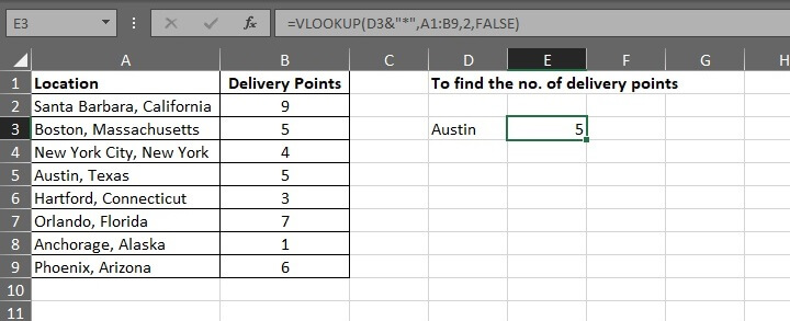 

2. FIND AND REPLACE

Using wildcard characters in Excel find and replace is beneficial to correct data and make the info set consistent throughout the database.

 This situation is especially common when handling data entered manually, either by staff or customers, creating extra values within the database and will make analysis difficult.

 The example below shows a standard picture when handling a client’s database.

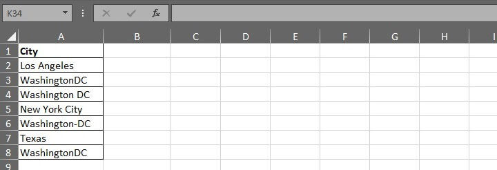The cities under Washington DC could be confusing.

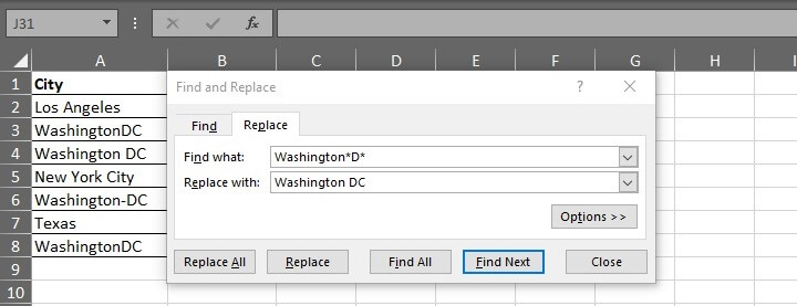
To rectify, use the straightforward  “FIND AND REPLACE” function in Excel.

• Find Washington with a D after it and replace it as “Washington DC” 

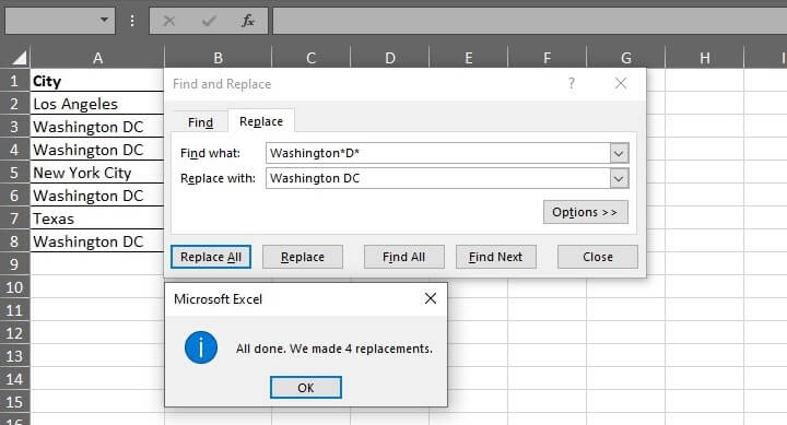
• Click “Replace All” and now all the “Washington DC” values are aligned, resulting in a clean database. 

3. COUNTIF

To include wildcard characters as a part of the COUNTIF function counts the amount of cells within the given range that meets the required number of characters.

i.e., there’s an inventory of country codes, and therefore the task is to count the amount of nations with three characters in their respective country code.

In this scenario, each ? refers to one character. 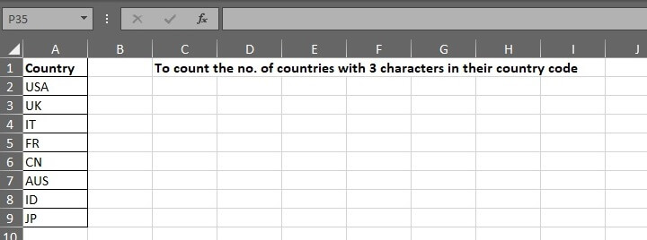Since we might wish to determine the country with three characters in their country code, the formula should include three ???

To find out, enter: 

=COUNTIF(A2:A9;"???")

The return value is 2.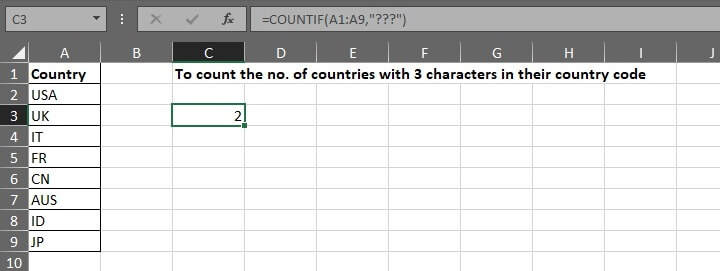 

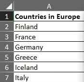
4. CONDITIONAL FORMATTING

In addition to formulas, wildcard characters are often wont to create conditional formatting also .

Say, the task is to spotlight the countries with names that begin with the letter G. 

1. Go to Conditional Formatting > New Rule > Select “Use a formula to determine which cells to format.”
2. Input the formula below. 

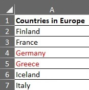
The idea is to find countries with names that begin with the letter G. So * (asterisk) is used to request Excel to return values that begin with G and are followed by any number of characters.

3. Select the desired formatting — in this case, font in red. 

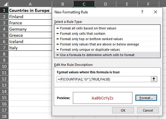
4. Click Okay, then apply the same format to the rest of the cells under Column A by using Format Painter. 

The result is below:

Excel wildcard not working? Here's why

Excel wildcard not working? Here's why
Mentioned previously, the utilization of * (asterisk) and ? (question mark) ask different situations. However, they don’t work if the wildcard characters themselves are a part of the lookup value.

• i.e., to find “Aus?”, “Aus~?” is required.

 

If you have any query or want any help related to excel feel free to join our Telegram channel and message us..

Channel link :

https://t.me/msexcelmaster101