How to apply negative vlookup to return the value in left of the key field in Excel?
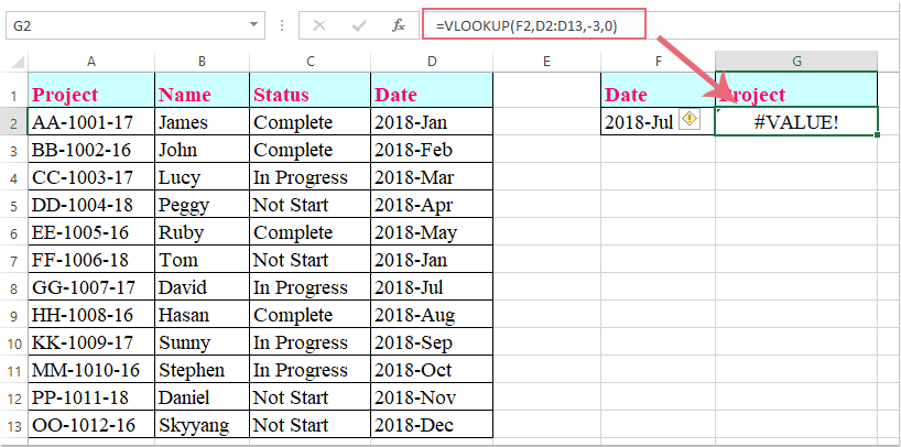
Normally, the Vlookup function can help you to return the value in right columns. If your extracted data in left column, you may consider entering a negative column number within the formula: =Vlookup(F2,D2:D13,-3,0), but this will give an error result as following screenshot shown. How could you apply negative vlookup function to return a matching value in Excel?

Apply negative vlookup to return the value in left column with User Defined function
The following User Defined Function can help you to apply the negative vlookup in Excel worksheet, please do as this:
1. Hold down the ALT + F11 keys to open the Microsoft Visual Basic for Applications window.
2. Click Insert > Module, and paste the following code in the Module window.
VBA code: Apply negative vlookup to return the value in left column:
Download VBA file (alternate link)
3. Then save and close the code window, go back to the worksheet, and enter this formula: =VLOOKUPNEG(F2,D2:D13,-3,0) into a cell where you want to get the result, and then press Enter key, and the matched value in left column has been extracted successfully, see screenshot:

Note: In the above formula, F2 is the cell contains the criteria you want to vlookup, D2:D13 is the column range where to search for, -3 is the column index number you want to return the matching value from.
If you have any query or want any help related to excel feel free to join our Telegram channel and message us..
Channel link :


0 Comments