Excel Basics tips and tricks (Part -1)
If you're just starting out with Excel, there are a few basic commands that we suggest you become familiar with. These are things like:
1. Use Pivot Tables to recognize and make sense of data.
Pivot Tables are used to reorganize data in a spreadsheet. They won't change the data that you have, but they can sum up values and compare different information in your spreadsheet, depending on what you'd like them to do.
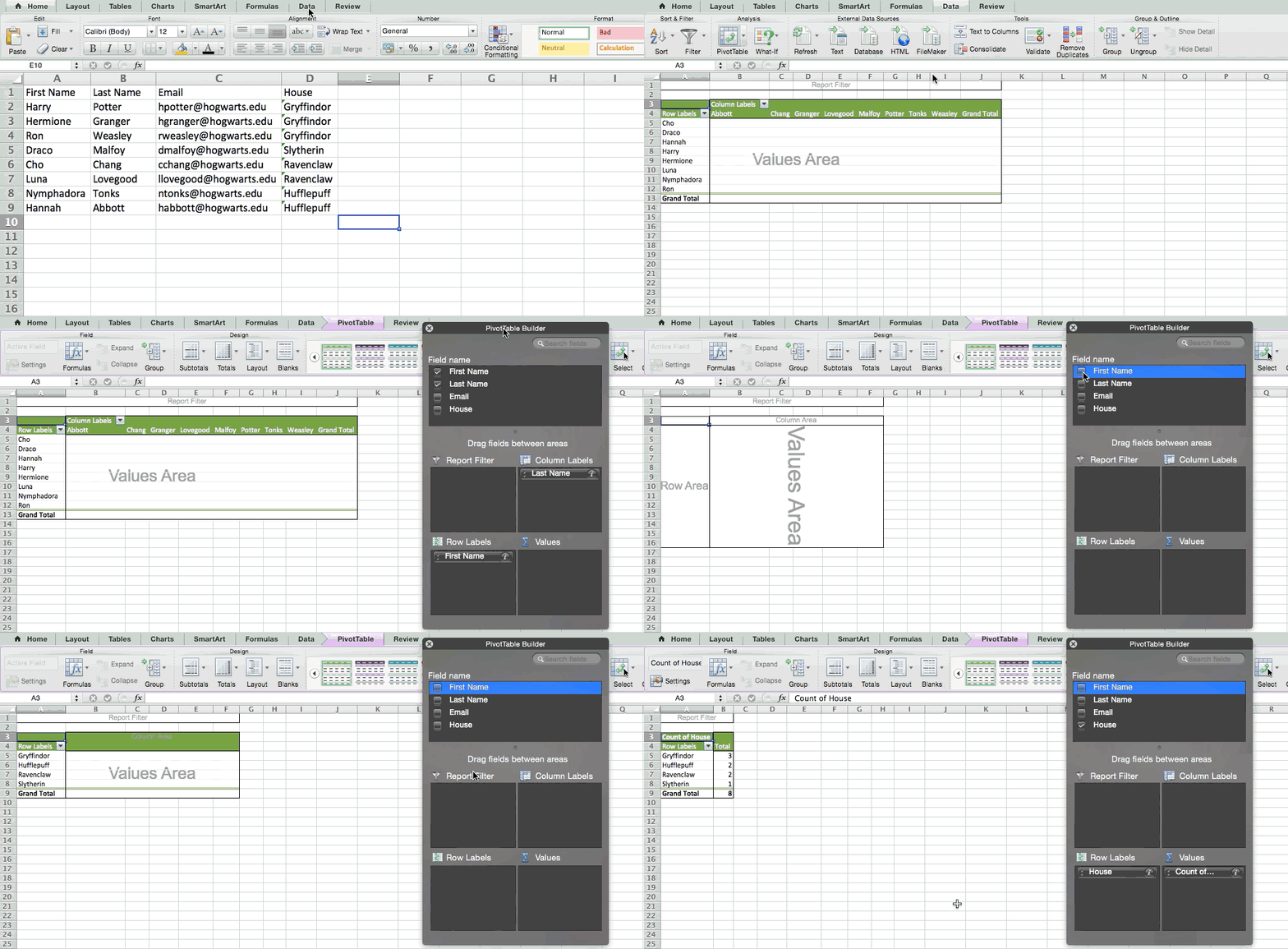
Let's take a look at an example. Let's say I want to take a look at how many people are in each house at Hogwarts. You may be thinking that I don't have too much data, but for longer data sets, this will come in handy.
To create the Pivot Table, I go to Data > Pivot Table. Excel will automatically populate your Pivot Table, but you can always change around the order of the data. Then, you have four options to choose from.
- Report Filter: This allows you to only look at certain rows in your dataset. For example, if I wanted to create a filter by house, I could choose to only include students in Gryffindor instead of all students.
- Column Labels: These could be your headers in the dataset.
- Row Labels: These could be your rows in the dataset. Both Row and Column labels can contain data from your columns (e.g. First Name can be dragged to either the Row or Column label -- it just depends on how you want to see the data.)
- Value: This section allows you to look at your data differently. Instead of just pulling in any numeric value, you can sum, count, average, max, min, count numbers, or do a few other manipulations with your data. In fact, by default, when you drag a field to Value, it always does a count.
Since I want to count the number of students in each house, I'll go to the Pivot Table and drag the House column to both the Row Labels and the Values. This will sum up the number of students associated with each house.
2. Use filters to simplify your data.
When you're looking at very large data sets, you don't usually need to be looking at every single row at the same time. Sometimes, you only want to look at data that fit into certain criteria. That's where filters come in.
Filters allow you to pare down your data to only look at certain rows at one time. In Excel, a filter can be added to each column in your data -- and from there, you can then choose which cells you want to view at once.
Let's take a look at the example below. Add a filter by clicking the Data tab and selecting "Filter." Clicking the arrow next to the column headers and you'll be able to choose whether you want your data to be organized in ascending or descending order, as well as which specific rows you want to show.
In my Harry Potter example, let's say I only want to see the students in Gryffindor. By selecting the Gryffindor filter, the other rows disappear.
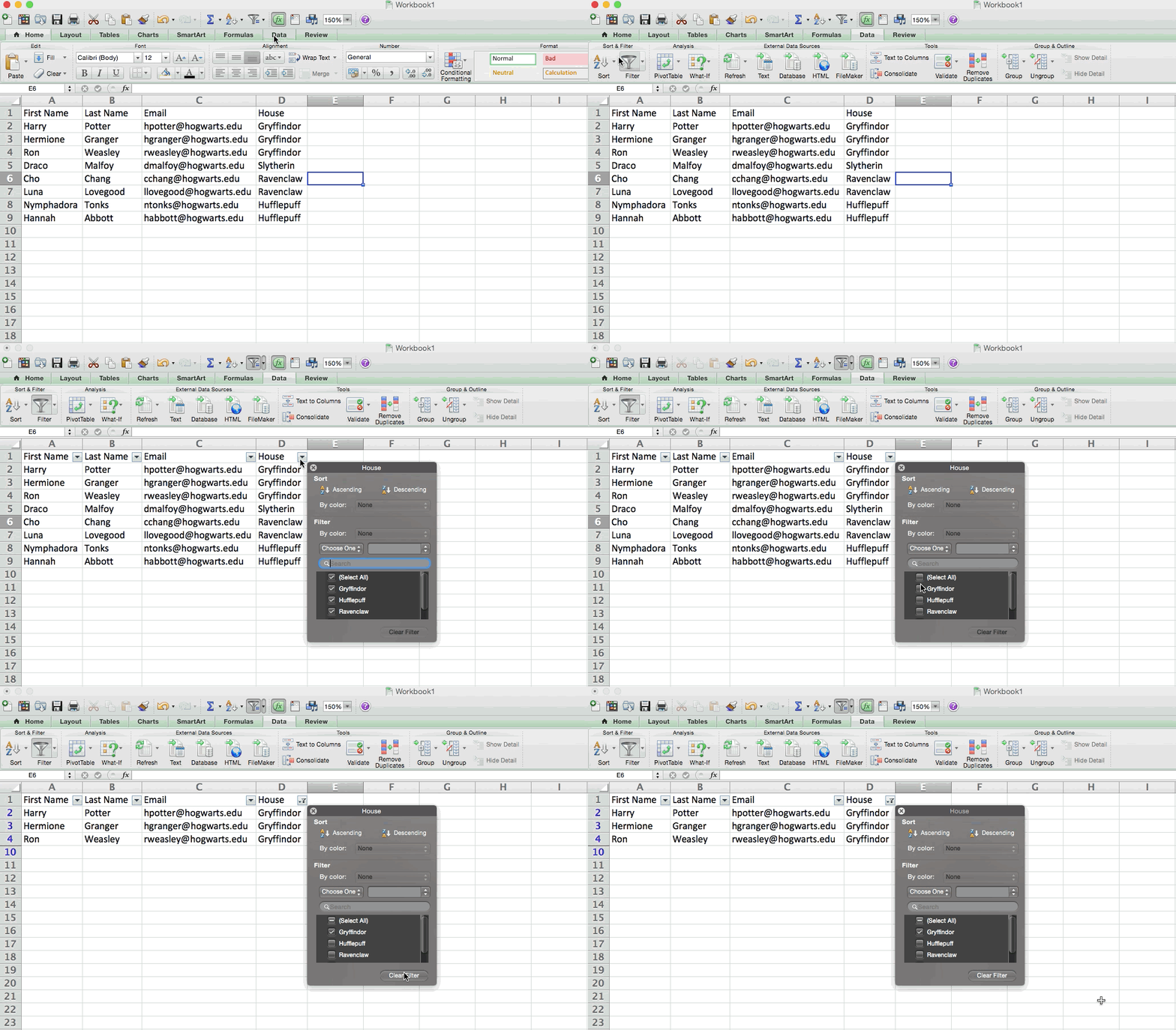
Pro Tip: Copy and paste the values in the spreadsheet when a Filter is on to do additional analysis in another spreadsheet.
3. Transpose rows into columns.
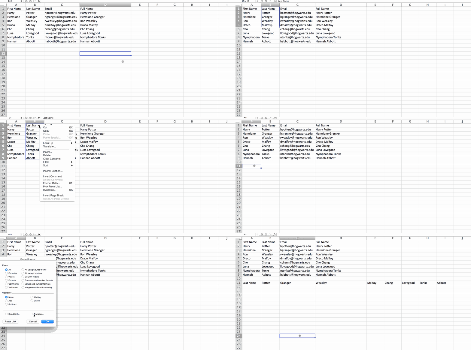
When you have low rows of data in your spreadsheet, you might decide you actually want to transform the items in one of those rows into columns (or vice versa). It would take a lot of time to copy and paste each individual header -- but what the transpose feature allows you to do is simply move your row data into columns, or the other way around.
Start by highlighting the column that you want to transpose into rows. Right-click it, and then select "Copy." Next, select the cells on your spreadsheet where you want your first row or column to begin. Right-click on the cell, and then select "Paste Special." A module will appear -- at the bottom, you'll see an option to transpose. Check that box and select OK. Your column will now be transferred to a row or vice-versa.
4. Use these formulas for simple calculations
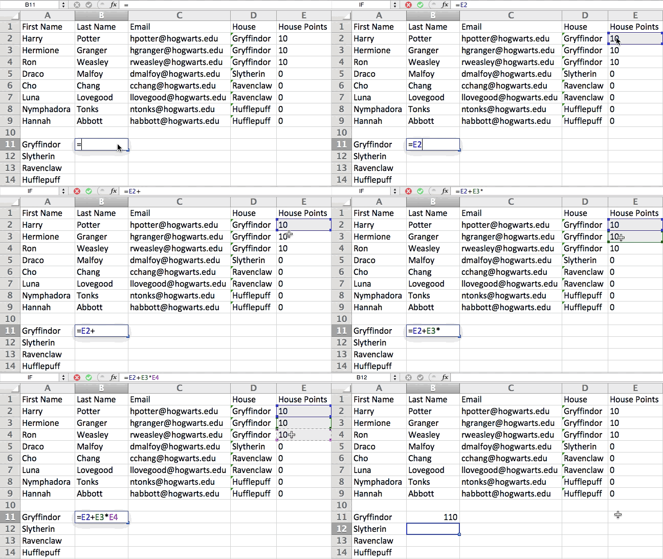
In addition to doing pretty complex calculations, Excel can help you do simple arithmetic like adding, subtracting, multiplying, or dividing any of your data.
- To add, use the + sign.
- To subtract, use the - sign.
- To multiply, use the * sign.
- To divide, use the / sign.
You can also use parenthesis to ensure certain calculations are done first. In the example below (10+10*10), the second and third 10 were multiplied together before adding the additional 10. However, if we made it (10+10)*10, the first and second 10 would be added together first.
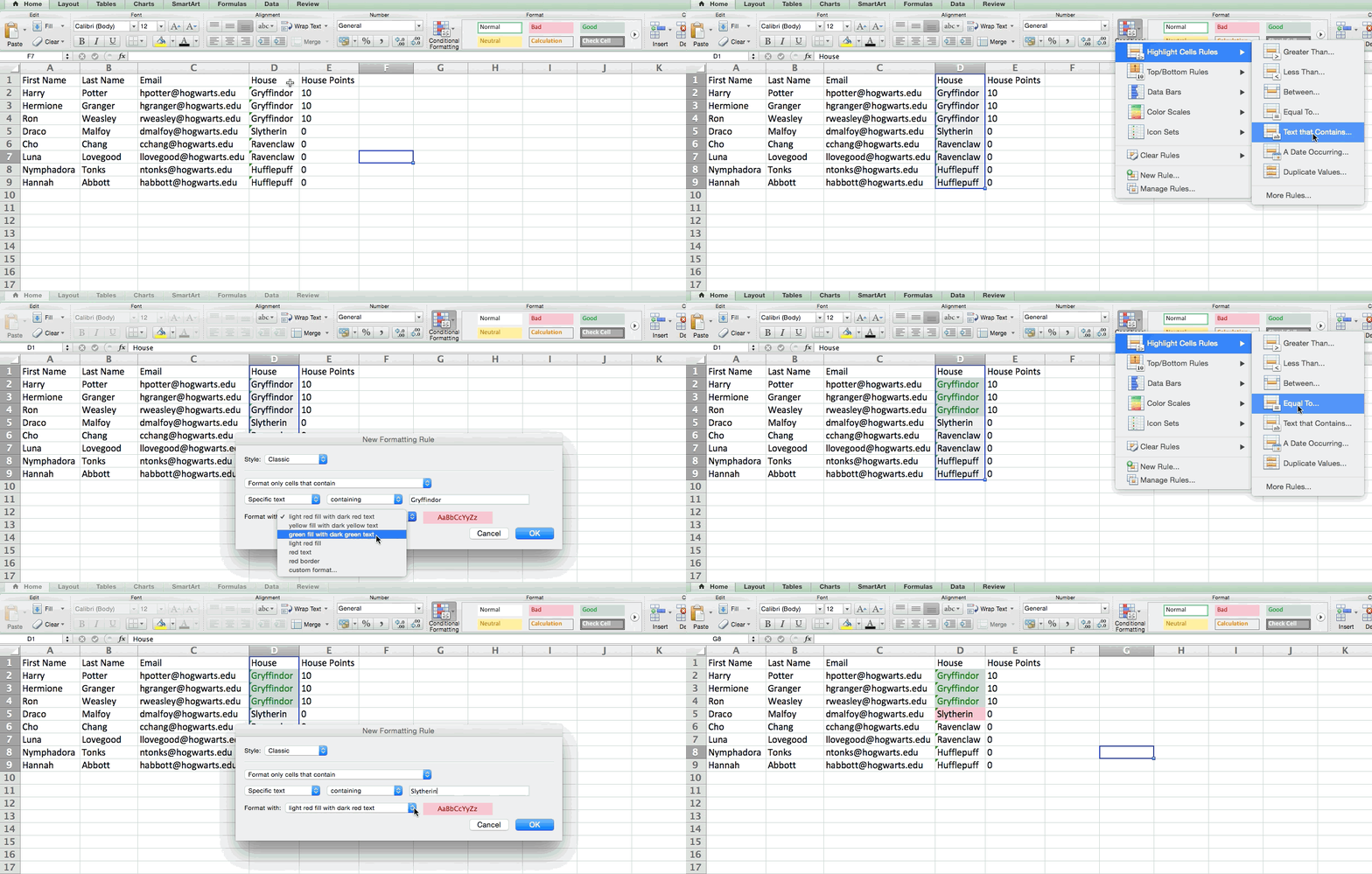
5. Use conditional formatting to make cells automatically change color based on data.
Conditional formatting allows you to change a cell's color based on the information within the cell. For example, if you want to flag certain numbers that are above average or in the top 10% of the data in your spreadsheet, you can do that. If you want to color code commonalities between different rows in Excel, you can do that. This will help you quickly see information the is important to you.
To get started, highlight the group of cells you want to use conditional formatting on. Then, choose "Conditional Formatting" from the Home menu and select your logic from the dropdown. (You can also create your own rule if you want something different.) A window will pop up that prompts you to provide more information about your formatting rule. Select "OK" when you're done, and you should see your results automatically appear.
6. Use dollar signs to keep one cell's formula the same regardless of where it moves.
Have you ever seen a dollar sign in an Excel formula? When used in a formula, it isn't representing an American dollar; instead, it makes sure that the exact column and row are held the same even if you copy the same formula in adjacent rows.
You see, a cell reference -- when you refer to cell A5 from cell C5, for example -- is relative by default. In that case, you're actually referring to a cell that's five columns to the left (C minus A) and in the same row (5). This is called a relative formula. When you copy a relative formula from one cell to another, it'll adjust the values in the formula based on where it's moved. But sometimes, we want those values to stay the same no matter whether they're moved around or not -- and we can do that by making the formula in the cell into what's called an absolute formula.
To change the relative formula (=A5+C5) into an absolute formula, we'd precede the row and column values by dollar signs, like this: (=$A$5+$C$5). (Learn more on Microsoft Office's support page here.)
Please comment if you like this tips and tricks..
Part-2 Coming Soon
If you have any query or want any help related to excel feel free to join our Telegram channel and message us..
Channel link :


0 Comments