
Consolidate Multiple Excel Sheets Using Power Query Append
One of the top questions I get from blog readers is if there is a way to easily consolidate multiple Excel worksheets into one.
With Power Query the answer is a big YES!
If you have multiple Excel worksheets that are in the same format and their underlying differences are their values and dates, then we can easily consolidate all the worksheets into one.
The crucial part here is it has to be in the same format so that we can append them together.
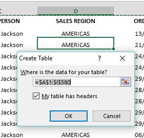
STEP 1: Make sure that each worksheet’s data is in an Excel Table by clicking in the data and pressing CTRL+T
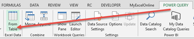
STEP 2: Click in each of the worksheets data that you want to consolidate and select:
Power Query > From Table
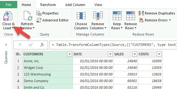
STEP 3: This will open up the Query Editor and all you have to do here is press Close & Load.
Make sure to do Steps 2 & 3 for each worksheet you want to consolidate. This will include load all our worksheets into Power Query.
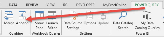
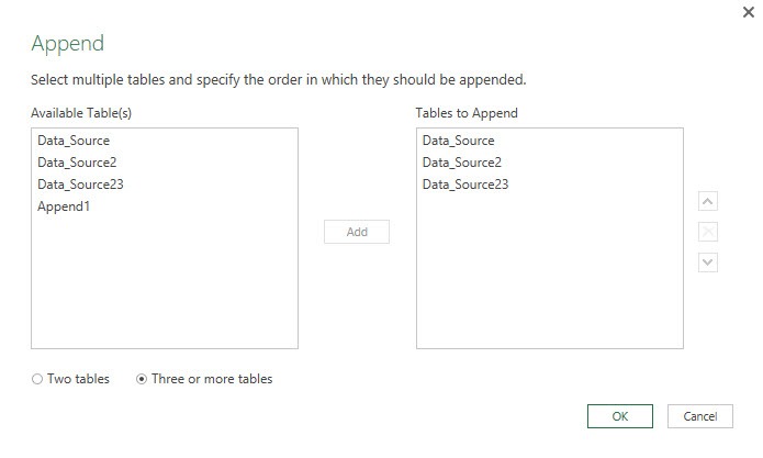
STEP 4: Select Power Query > Append
STEP 5: Choose the Three or more tables option

STEP 6: Add the tables to append from the Available Tables (from the left) to the Tables to Append (to the right) by selecting and pressing the Add button.
You can also organize the order that you want your consolidated table to appear by moving the Tables up or down.
So your merged table will be a combination of the tables listed on the right.
Press the OK button!
STEP 7: This will open up the Query Editor once again. Choose Close & Load.
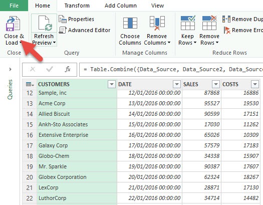
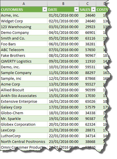
STEP 8: This will open up a brand new worksheet which will consolidate all the worksheets into one big Table.
No more manual copy and pasting! If the underlying tables get their data updated, this Power Query result will retrieve these changes as well when you do a refresh!
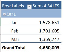
STEP 9: From this consolidated worksheet you can Insert a Pivot Table and do your analysis:
Linking Excel Tables in Power Pivot
When you have multiple tables, Power Pivot can help you link them together. After linking them together you can then create a Pivot Table that will give you a single view of data.
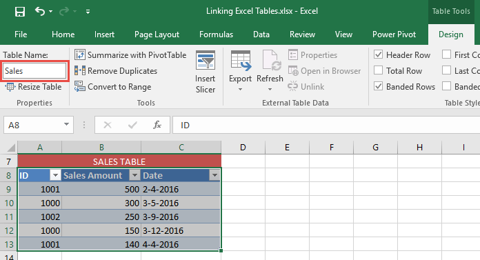
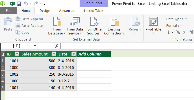
What we will focus on is a simple example of two Excel Tables: a Name Table and a Sales Table.
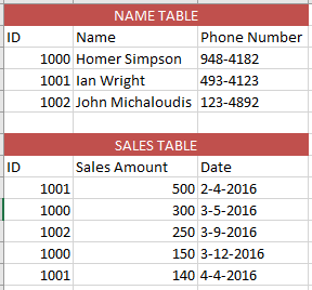
What we want to know is how much each Employee made in Total Sales.
You can see that each employee is uniquely identified by the ID number, which is also used in the Sales table. This is a crucial identifier for us to relate the two tables together.
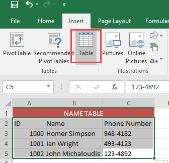
STEP 1: Select your first table. Go to Insert > Table. Click OK.
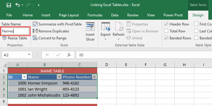
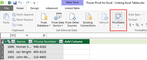
STEP 2: Go to Design > Table Name and give your Table a descriptive name. In our example, we will name it Names
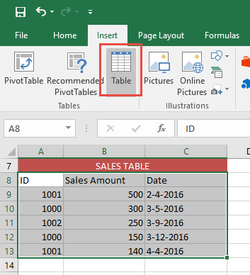
STEP 3: Select your second table. Go to Insert > Table. Click OK.
STEP 4: Go to Design > Table Name and give your Table a descriptive name. In our example, we will name it Sales
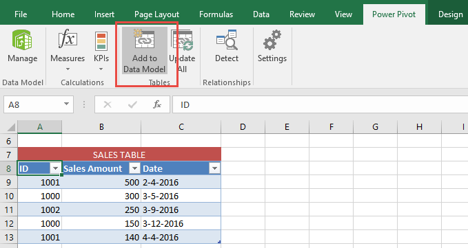
STEP 5: Select your first table. Go to Power Pivot > Add to Data Model. This will import your new Table into the Power Pivot Window.
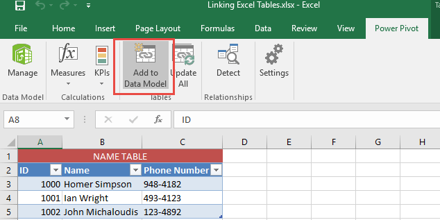
STEP 6: Select your second table. Go to Power Pivot > Add to Data Model. This will import your new Table into the Power Pivot Window.
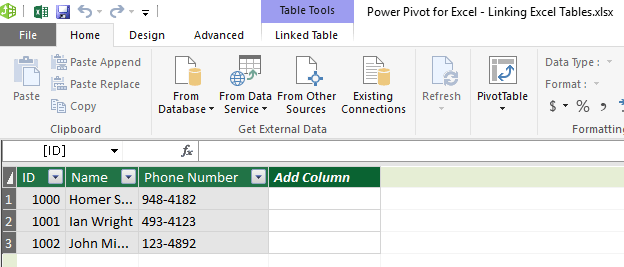
STEP 7: This will open the Power Pivot Window. Your two Tables should already be loaded there.
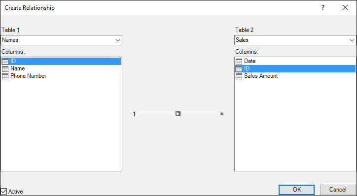
STEP 8: Go to Design > Create Relationship.
What will define our relationship? It will be the ID column linking these two tables together.

STEP 9: Ensure for Table 1, you set Names = ID and for Table 2, you set it to Sales = ID.
This will set the relationship and your Sales table will be able to see the values in the Names table.
STEP 10: With this, our setup is complete. Now it’s time to create a Pivot Table to do our analysis!
You will be excited to see how our Pivot Table will be able to use the data from two tables simulatenously!
Within the PowerPivot Window, go to Home > PivotTable.
Select New/Existing Worksheet and press OK
STEP 11: This will create a new Pivot Table within your Excel worksheet.
We will get information from both tables! Without any additional setup needed because we have put the relationship in place.
In the ROWS area put in the Name field from the Names Table, in the VALUES area you need to put in the Sales Amount field from the Sales Table:
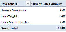
STEP 12: We now have the Names and the Total Sales Amount all in one Pivot Table.
We were able to link and consolidate two Excel Tables together with no need for Vlookup or helper columns…thanks to Power Pivot!
If you have any query or want any help related to excel feel free to join our Telegram channel and message us..
Channel link :

2 Comments
I had query related to merging many excel spreadsheet, but your post have solved every thing.
ReplyDeleteGreat Work man
Thank you😊
Delete